Lab 7 - Kalman Filtering

Posted on 2026-03-25

Sensor Debugging

Before driving anything I verified both ToF sensors were working. The front sensor (distanceSensor2) read ~1392mm to the wall, the side sensor read ~93mm. Both at ~10 Hz, Short mode.

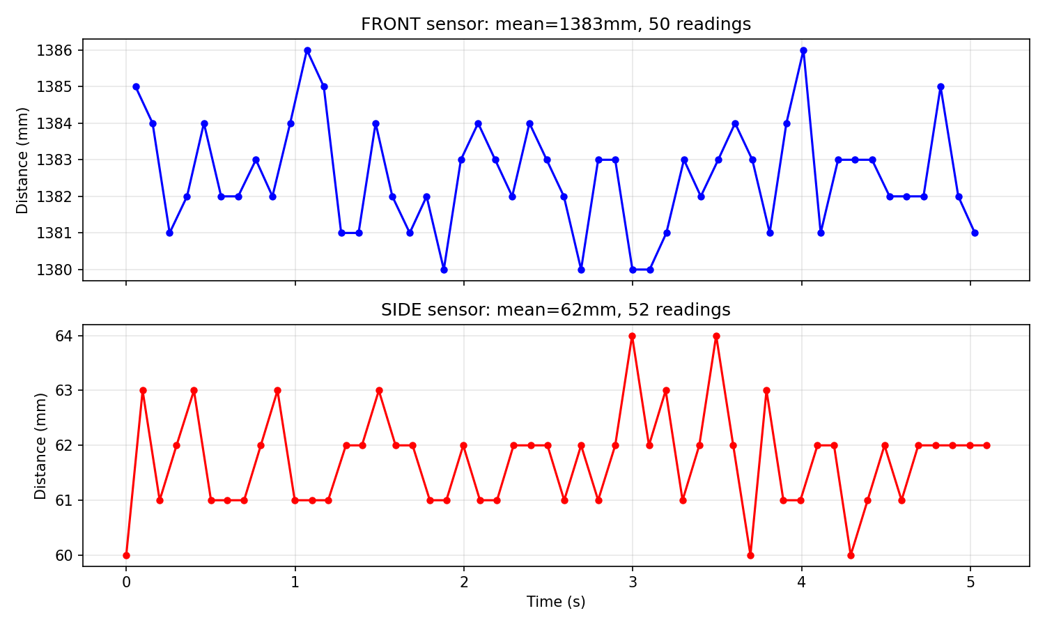
Both ToF sensors verified before step response testing.

1. Estimate Drag and Momentum

I added a BLE command to drive at constant PWM while logging ToF data. This way I can set the PWM and duration from Jupyter without re-uploading.

ble.send_command(CMD.SET_PID_DURATION, "5000")
ble.send_command(CMD.SET_CALIBRATION, "3.5")
ble.send_command(CMD.START_STEP_RESPONSE, "60")

I used PWM=60 (with calibration=3.5 on the left motor to go straight). Started about 1.4m from the wall with foam padding. First attempt at PWM=120 was way too fast, the car flipped on its back.

Open video if it doesn't play above.

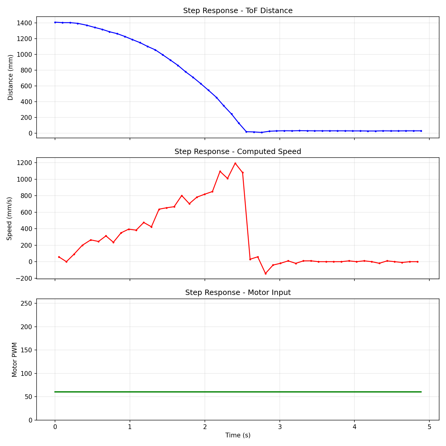
Step response: ToF distance, computed speed, and motor input. The car hit the wall at ~2.5s.

The car hit the wall before reaching steady state so the exponential curve fit gave an unreasonable v_ss of 11 million mm/s. Instead I estimated manually: took the max pre-impact speed (1194 mm/s), bumped it by 20% since it was still climbing, giving v_ss = 1433 mm/s. I found when the speed crossed 60% of v_ss (at t=2.20s) and scaled to get t_90 = 5.54s.

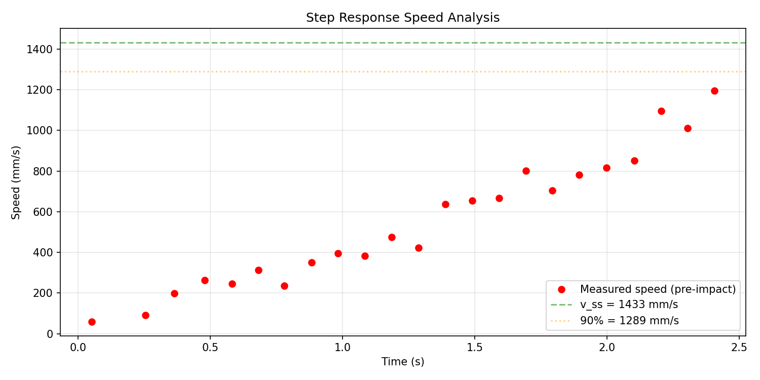
Speed vs time with estimated steady-state and 90% lines.

From these: d = 0.000698, m = 0.001679. Data saved to CSV.

2. Initialize KF

State is [distance (mm), velocity (mm/s)]. One important thing: positive motor command drives toward the wall (distance decreases), so I negate the input when feeding it to the KF.

A = np.array([[0, 1],
              [0, -d/m]])   # [[0, 1], [0, -0.416]]
B = np.array([[0],
              [1/m]])       # [[0], [595.7]]
C = np.array([[1, 0]])

# Discretize at actual dt between samples
Ad = np.eye(2) + dt * A
Bd = dt * B

# Process noise
Sigma_u = np.diag([20**2, 40**2])   # position, velocity
# Sensor noise (VL53L1X Short mode datasheet)
Sigma_z = np.array([[20**2]])

I set position process noise to 20mm and velocity to 40mm/s as starting points. Sensor noise is 20mm from the VL53L1X datasheet for Short mode. These balance trusting the model vs sensor roughly equally.

3. KF in Jupyter

I ran the KF on a fresh PID run (285 samples, 24 ToF readings over 2.37s). The filter predicts every loop iteration and updates only when a new ToF reading arrives.

def kf(mu, sigma, u, y, has_measurement, dt):
    Ad = np.eye(2) + dt * A
    Bd = dt * B

    mu_p = Ad @ mu + Bd * u
    sigma_p = Ad @ sigma @ Ad.T + Sigma_u

    if has_measurement:
        S = C @ sigma_p @ C.T + Sigma_z
        K = sigma_p @ C.T @ np.linalg.inv(S)
        y_m = np.array([[y]]) - C @ mu_p
        mu = mu_p + K @ y_m
        sigma = (np.eye(2) - K @ C) @ sigma_p
    else:
        mu = mu_p
        sigma = sigma_p
    return mu, sigma

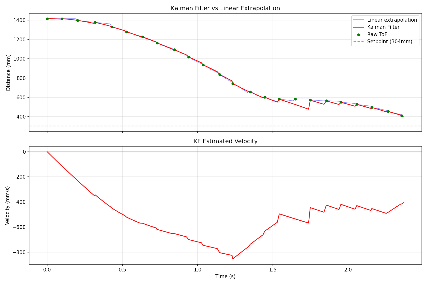
KF estimate (red) vs linear extrapolation (blue) vs raw ToF readings (green). Both track well, KF is smoother.

The KF tracks the raw ToF data smoothly and provides a velocity estimate. It performs similarly to linear extrapolation on this data but the real advantage is the velocity state which the extrapolation doesn’t give.

To sanity check the dynamics model I set sensor noise astronomically high (1e8) so the KF ignores sensor data and runs purely on the model. It tracks the actual trajectory for the first ~1.5s then diverges when PID starts braking, which makes sense since the model doesn’t know about the control input changing.

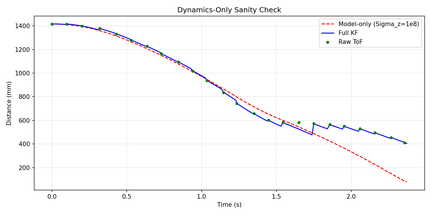
Model-only prediction (red dashed) vs full KF (blue). Model diverges when PID brakes, which is expected.

4. KF on the Robot

I implemented the KF on the Artemis using the BasicLinearAlgebra library. All parameters (d, m, sigma values) are sent from Jupyter via BLE so I can tune without re-uploading.

void kf_predict(float u_norm, float dt_s) {
    Matrix<2,2> Ad = {1, dt_s,
                      0, 1 - (kf_d/kf_m) * dt_s};
    Matrix<2,1> Bd = {0, dt_s / kf_m};
    Matrix<1> u_mat = {u_norm};
    x_kf = Ad * x_kf + Bd * u_mat;
    P_kf = Ad * P_kf * ~Ad + Sigma_u_kf;
}

void kf_update(float measurement) {
    Matrix<1,2> C_kf = {1, 0};
    Matrix<1,1> S = C_kf * P_kf * ~C_kf + Sigma_z_kf;
    Matrix<2,1> K = P_kf * ~C_kf * Inverse(S);
    Matrix<1,1> y_err = {measurement - (C_kf * x_kf)(0)};
    x_kf = x_kf + K * y_err;
    Matrix<2,2> I = {1, 0, 0, 1};
    P_kf = (I - K * C_kf) * P_kf;
}

The PID loop calls kf_predict every iteration and kf_update only when a new ToF reading arrives. I kept linear extrapolation as a fallback toggled by a BLE command.

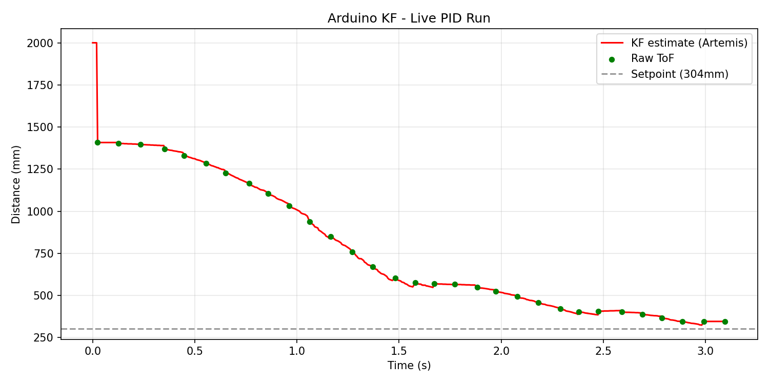
KF running on the Artemis during a live PID run. Smooth tracking through 31 ToF readings down to the 304mm setpoint. The initial spike to 2000mm is the default distance before the first sensor reading arrives.