Lab 12 - Inverted Pendulum (Wheelie)

Setup

For the final lab I picked Lab 12b, the inverted pendulum, over the path planning option. The control side of the class has been more fun to flex than the planning side, and I had nearly everything I needed already from Lab 2 (DMP), Lab 6 (PD pattern), and Lab 7 (Kalman pattern) to build on. The lab is also intentionally wide open, you just need to make the car stand on its rear wheels and keep it there.

I was directly inspired by the Nita Kattimani, Aravind Ramaswami, and Anunth Ramaswami project from a previous year. They built a Lagrangian model of the car-as-pendulum, used MATLAB pole placement to pick the gains, fused angle and angular velocity with a Kalman filter, and ran a hard-coded state machine that flipped the car off the floor and handed it to the balance controller. That writeup gave me the right vocabulary (alpha1, alpha2, the state-space form) and I copied parts of their structure even though my implementation ended up simpler.

Honestly this was the most fun lab of the semester. There is something genuinely satisfying about feeling out a balance point by hand, calibrating the IMU against it, and then watching the car catch its own fall a few minutes later.

1. Physical measurements and dynamics

The cart-pole model wants five numbers (plus gravity). I weighed both halves of the car separately and pulled out the rear wheels for the inertia measurement.

M (rear wheels)              = 138.0 g
m (body + front wheels)      = 398.0 g
l (rear axle to body COM)    = 6.1 cm
r (rear wheel radius)        = 3.9 cm

For the moment of inertia I hung the body from the rear axle on two strings and timed swings as a physical pendulum:

Three trials of 10 swings each, dropped one as a clear outlier. Averaging the two clean trials gave $T = 1.020$ s and $I_{pivot} = 0.00629$ kg·m².

Plugging into the linearized cart-pole alpha coefficients:

For comparison, the reference team had $\alpha_1 = 6.21$. My car falls roughly $\sqrt{46/6.21} \approx 2.7$ times faster than theirs, with a natural falling time around 0.15 s vs their 0.40 s. That immediately told me their pole-placement gains would not transfer to my car, and I would need to react more aggressively.

2. Pitch from the DMP (with mounting calibration)

Lab 6 already had the DMP running, dumping a quaternion every ~18 ms. I needed pitch instead of yaw. The standard ZYX Euler pitch formula asin(2(q0q2 − q3q1)) was the obvious choice but gave wrong readings on my car. A three position sweep returned -46° flat, -76° at a 45° tilt, and -44° upright. Non-monotonic and compressed (only ~30° of swing for 90° of physical rotation), because my chip is mounted at a weird compound angle and the car’s pitch motion projects onto multiple chip axes.

I switched to a mounting-independent approach using two calibration snapshots. With the car flat I snapshot the chip’s “up” direction as g_flat, and with the car upright I snapshot as g_upright. Both come from the third row of the quaternion’s rotation matrix:

current_up[0] = 2.0 * (q1*q3 - q0*q2);
current_up[1] = 2.0 * (q2*q3 + q0*q1);
current_up[2] = 1.0 - 2.0 * (q1*q1 + q2*q2);

At runtime, the pitch is the angle between the current “up” and the two calibrated references, projected onto the plane they span:

float dot_flat    = current_up[0]*g_flat[0]    + current_up[1]*g_flat[1]    + current_up[2]*g_flat[2];
float dot_upright = current_up[0]*g_upright[0] + current_up[1]*g_upright[1] + current_up[2]*g_upright[2];
current_pitch     = atan2(dot_upright, dot_flat) * 180.0 / M_PI;

After recalibrating with this method the three position sweep returned 1.1°, 49.5°, and 88.6°. Monotonic, linearly spaced, and the upright reading matched what the accelerometer had given me earlier as $\theta_{eq}$.

3. Pitch rate via gyro projection

For the D term I wanted true rate of car pitch, not a single gyro axis. Because of the mounting, no single gyro axis is “the pitch rate.” Luckily the calibration also gives the actual pitch axis as the cross product of the two reference vectors:

Then the rate is the dot product of the raw gyro vector with this axis:

current_pitch_rate = gyrX*pitch_axis[0]
                   + gyrY*pitch_axis[1]
                   + gyrZ*pitch_axis[2];

Moving the car from flat to upright by hand produced clean rate peaks around ±150 dps with the right sign, no compression, no axis ambiguity.

4. Balance controller

The controller is a PD loop firing on each DMP update (~56 Hz). With the linearized dynamics $\ddot{\theta} = \alpha_1 \theta - \alpha_2 u$ and u = Kp·error + Kd·rate, the closed-loop equation is

This is a damped spring, so I pick a target natural frequency $\omega_n$ and damping ratio $\zeta$, then solve:

With $\omega_n = 10$ rad/s (about 1.5× the unstable mode) and $\zeta = 0.7$, I got $K_p \approx 0.65$ and $K_d \approx 0.06$ in physical (torque) units. Converting through a rough Lab 7 torque-per-PWM estimate landed at starting gains $K_p \approx 6$ PWM/deg and $K_d \approx 0.6$ PWM/(deg/s).

The Arduino loop, with a safety threshold and a deadband bump for the motor’s friction band:

if (dmp_data_ready) {
    float error = current_pitch - balance_setpoint;
    if (fabs(error) > balance_safety_threshold) {
        balance_running = false;
        stop_motors();
    } else {
        float u = balance_kp * error + balance_kd * current_pitch_rate;
        int motor_cmd = constrain((int)u, -balance_max_pwm, balance_max_pwm);
        if (motor_cmd > 0 && motor_cmd <  balance_deadband) motor_cmd =  balance_deadband;
        if (motor_cmd < 0 && motor_cmd > -balance_deadband) motor_cmd = -balance_deadband;
        // analogWrite both wheels at |motor_cmd|, direction from sign(motor_cmd)
    }
}

The setpoint is computed automatically from the two calibration vectors (88.6° for my upright). Safety threshold is 30° from setpoint, motors kill the moment the car has clearly fallen.

5. Tuning trials

Trial 1. First real attempt at the derived $K_p = 6$, $K_d = 0.6$, deadband = 60. The motor sign turned out to be flipped for my wiring so I switched to $K_p = -6$ for the rest. The car balanced for short stretches but kept falling forward, motor saturating at ±150 frequently.

Trial 1: first attempt with the derived gains, balance for a couple seconds before falling forward.

Trial 2. I dropped the deadband bump to 50 and bumped gains slightly to $K_p = -7$, $K_d = 0.7$. The car was noticeably more stable, held the balance through several obstacle hits in my room, but still drifted forward and eventually crashed.

Trial 2: improved stability after deadband and gain tuning, survived a few wall taps.

Trial 3 (final). Same gains as trial 2, but I started the car already at the balance angle by hand and released. The controller corrected the initial wobble and held the wheelie for several seconds.

Trial 3: hand-released into balance, several seconds of self-corrected wheelie.

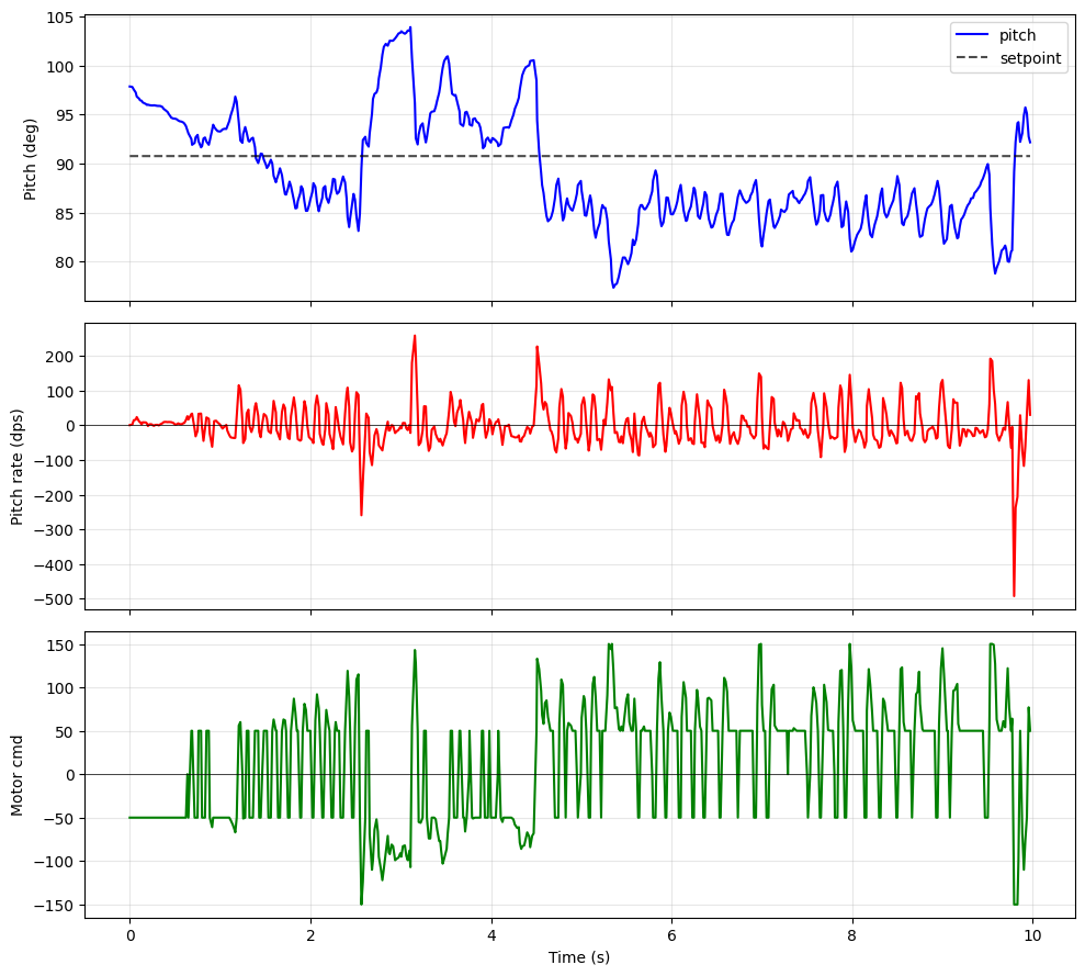
Trial 3 logged data: pitch tracks the 88.6° setpoint within roughly ±3° for most of the run. The motor command oscillates between ±150 with the deadband bump visible as flat segments around ±50.

6. What I couldn’t get to work (dynamic flip)

The remote-control version of my car can flip itself with a fast forward, hard reverse motion. I tried to recreate that with a timed open-loop sequence (forward 300 ms at PWM 255, reverse 250 ms at PWM 255, then hand to the balance controller). The car drove forward and back energetically but never actually tipped onto its rear wheels. I think the BLE latency between commands smears the transition timing enough that the inertia mechanism that works for a human-operated remote control just does not hit the right window when scripted.

The obvious next step is to move the state machine onto the Arduino so it can watch the live pitch and switch from FORWARD to REVERSE to BALANCE on a pitch threshold rather than fixed durations, the way the reference team’s project did it. I ran out of time before getting there.

7. Reflections

A couple of things I learned:

The forward drift of the balanced car is not a bug, it is a fundamental property of single-DOF pendulum control. To keep the body upright the wheels have to push under it, so the wheels accumulate translational velocity. Past student demos all show this same drift. Fixing it cleanly would need either a position sensor on the wheels or an integral term that learns “the car keeps leaning forward, push back a bit more.”

The Kalman filter the reference team used was tempting but not needed for my version. The DMP fuses gyro and accelerometer internally, and the pitch rate from the gyro projection was already clean enough that a PD controller could use it directly. I would only reach for a KF if the rate signal had real noise to filter out, which it did not.

Calibration accuracy was more important than I expected. The first time I calibrated CAL_PITCH_UPRIGHT with the car not actually at its real balance point, every downstream pitch reading was biased, and the balance controller tried to hold the car at the wrong angle. Recalibrating with the car held at the true static balance point fixed it.

Final best run: trial 3, several seconds of self-corrected balance from a hand-placed start, pitch held within ±3° of the calibrated 88.6° setpoint.