Lab 11 - Localization (real)

Setup

Lab 11 is the real-robot version of Lab 10. Only the update step of the Bayes filter runs at each pose, because the robot’s odometry is too noisy to be useful in the prediction step. At each marked pose I do one in-place 360° rotation, collect 18 ToF readings spaced 20° apart, and the filter compares those against pre-cached ray casts on the 12 by 9 by 18 grid to localize me.

I also added one new BLE command, OPEN_LOOP_SPIN(left_pwm, right_pwm, duration_ms[, reset]) (cmd 46). It drives LEFT_BWD and RIGHT_FWD directly at the configured PWMs (CCW), bypassing both the straight-line calibration that drive() applies and the setpoint mechanics of the yaw PID. DMP yaw and ToF logging keep running independently so the spin is captured. The optional reset flag (default 1) controls whether the yaw log resets at the start of the spin, which I needed for the burst pattern below.

1. Sim baseline

I ran lab11_sim.ipynb end-to-end first to confirm the provided Localization class still works on the virtual robot. Through the full 16-step trajectory the belief argmax (blue) stays glued to ground truth (green), the two traces overlap almost cell-for-cell around the loop. Odometry (red) drifts away after a few steps and ends up near (0, -4), well outside the map. That mismatch is the whole reason Lab 11 skips the prediction step on the real robot: the sensor model carries the localization, the motion model just adds noise.

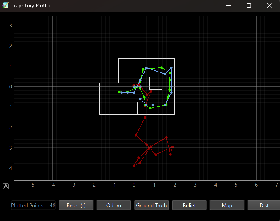
Final plot from the sim run: ground truth (green), odometry (red), belief argmax (blue). Belief tracks GT tightly even as odom diverges.

2. Observation loop on the real robot

Lab 9 taught me that PID-on-orientation stalls when small angle errors put the output below the deadband, so for Lab 11 I went open-loop. The first thing I tried was one long spin at fixed PWMs, but two problems showed up at home before lab.

The first problem was speed. At L=200, R=120, duration=12000ms the car spun about 4 full rotations, way more than I needed and way too fast for the ToF (~19 Hz) to fill all 18 bins. Three bins came back empty and the polar plot was missing chunks.

The second problem was drift. Even at slower PWMs the car translated a few inches off its starting spot during the spin, because the wheel speeds were not balanced enough for pure rotation.

I fixed both at once by switching to a burst pattern: 18 short spins at L=R=95, duration=500ms, with a 1 second rest between each. The short pulses don’t let translational momentum build up so the car stays nearly in place, and the long total time gives the ToF plenty of samples to populate every angle bin. To make the yaw log behave across the bursts I added a reset flag to OPEN_LOOP_SPIN. Burst 0 sends reset=1 to zero the log, the other 17 bursts send reset=0 so the yaw trace accumulates into one continuous 0 to ~600° curve.

There was also a Windows specific gotcha I had to fix. After SEND_YAW_PID_DATA the Python code was sleeping with time.sleep, but bleak dispatches BLE notifications on the asyncio event loop, and time.sleep blocks that loop. Notifications would queue silently during the wait and only fire after the cell ended, so parse_buffer saw 1 yaw row instead of 28. Switching to await asyncio.sleep (wrapped in a wait_for_drain helper) lets the loop pump and the notifications stream in correctly.

The Python side ended up short:

def perform_observation_loop(self, rot_vel=120):
    self.collected_data.clear()
    self.ble.send_command(CMD.START_TOF_DATA, '')
    time.sleep(0.2)

    for i in range(N_BURSTS):           # 18 bursts, 500 ms each, ~1 s rest between
        reset = 1 if i == 0 else 0
        self.ble.send_command(
            CMD.OPEN_LOOP_SPIN,
            f'{LEFT_PWM}|{RIGHT_PWM}|{DURATION_MS}|{reset}'
        )
        time.sleep(DURATION_MS / 1000 + REST_S)

    self.ble.send_command(CMD.STOP_TOF_DATA, '')
    time.sleep(0.3)
    self.ble.send_command(CMD.SEND_TOF_DATA, '')
    wait_for_drain(self.collected_data)
    self.ble.send_command(CMD.SEND_YAW_PID_DATA, '')
    wait_for_drain(self.collected_data)

    yaw_log, tof_log = parse_buffer(self.collected_data)
    readings = binned_observation(yaw_log, tof_log, n_bins=18, sensor='front')
    sensor_ranges = np.array(fill_nan_bins(readings))[np.newaxis].T
    return sensor_ranges, np.array([])

binned_observation interpolates yaw at each ToF timestamp, wraps it to [0, 360), assigns the sample to the nearest 20° bin, and takes the median per bin. Empty bins get filled with the world max range so the Gaussian in update_step does not blow up. I sanity checked the whole pipeline at home by placing the car inside a 6”×6” cardboard “room”, running the burst pattern, and projecting the 18 binned readings into world coordinates against the actual world.yaml walls. The points formed the expected ring around the origin with diagonals further than cardinals and all 18 bins populated.

One full burst-pattern 360° rotation in place.

3. Localization at the four marked poses

For each pose I placed the car at the marked tile with the nose pointing along +x (theta = 0), set robot.gt_pose accordingly, ran the observation loop and the update step once, and screenshotted the plotter.

Pose 1: (-3 ft, -2 ft, 0°)

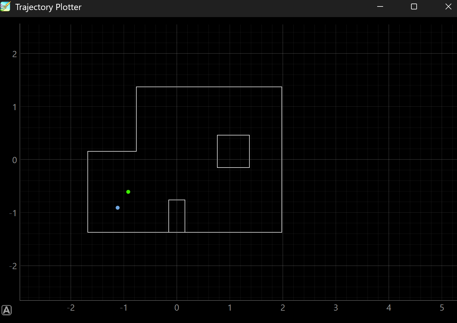
Belief (blue) one cell down-left of GT (green) at (-3 ft, -2 ft).

GT in meters is (-0.914, -0.610) which falls in grid cell (2, 2). The argmax belief came back at (-1.10, -0.90), cell (1, 1), so off by one cell in both x and y. Total Euclidean error around 0.36 m. This is the kind of off-by-one I expected from Lab 10 results, the bottom-left corner of the L is reasonably distinct but the walls along the lower edge do introduce some symmetry along x.

Pose 2: (0 ft, 3 ft, 0°)

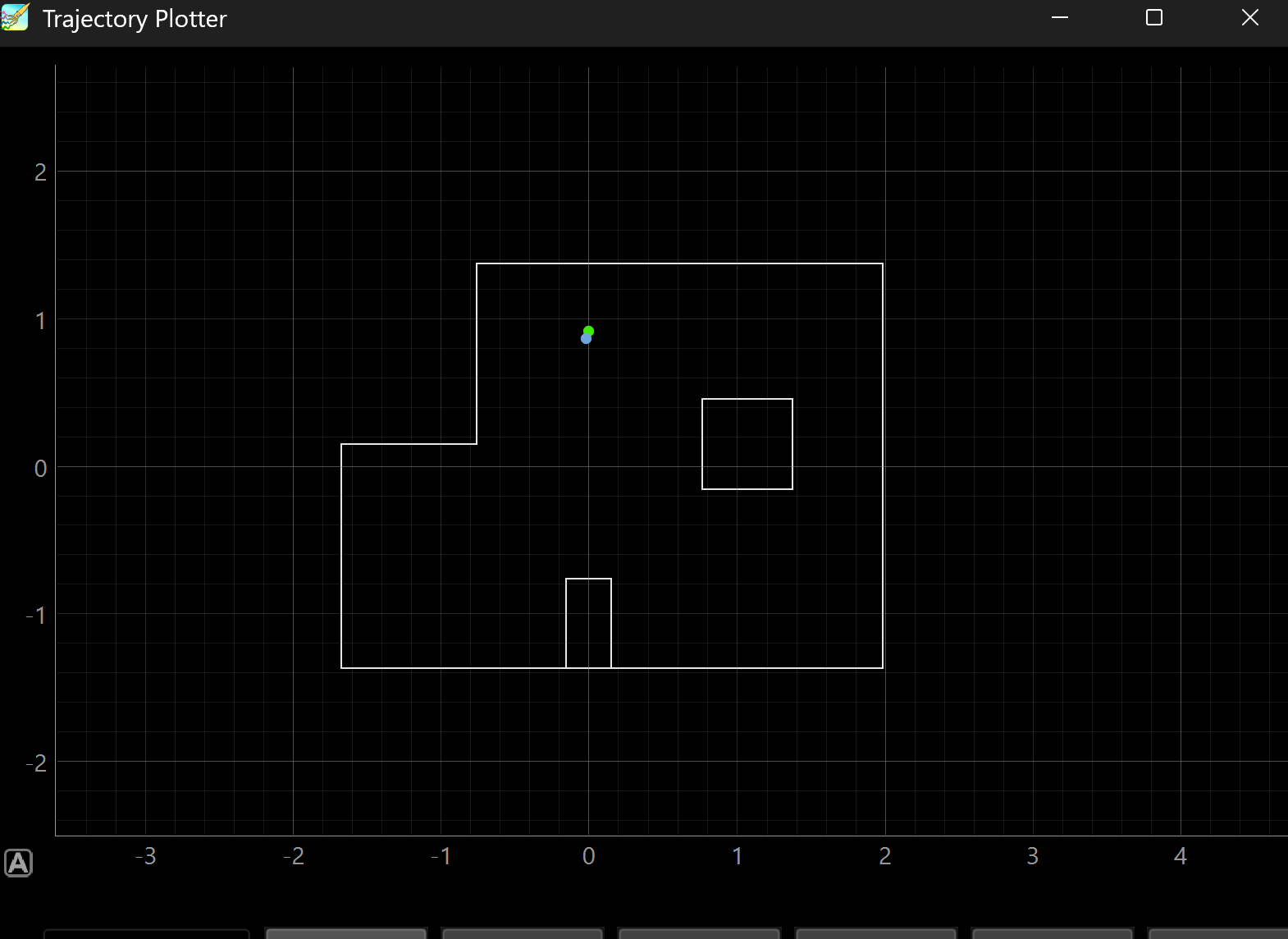
Belief sits exactly on GT inside the upper notch of the L.

GT (0.000, 0.914), cell (5, 7). Belief came back on the same cell, blue dot directly under the green one. This was the cleanest of the four. The pose sits inside the narrow upper part of the L which gives a very distinct ToF fingerprint, the close walls on the left and below dominate the sensor model and there is no symmetric pose anywhere else in the map that produces those readings.

Pose 3: (5 ft, -3 ft, 0°)

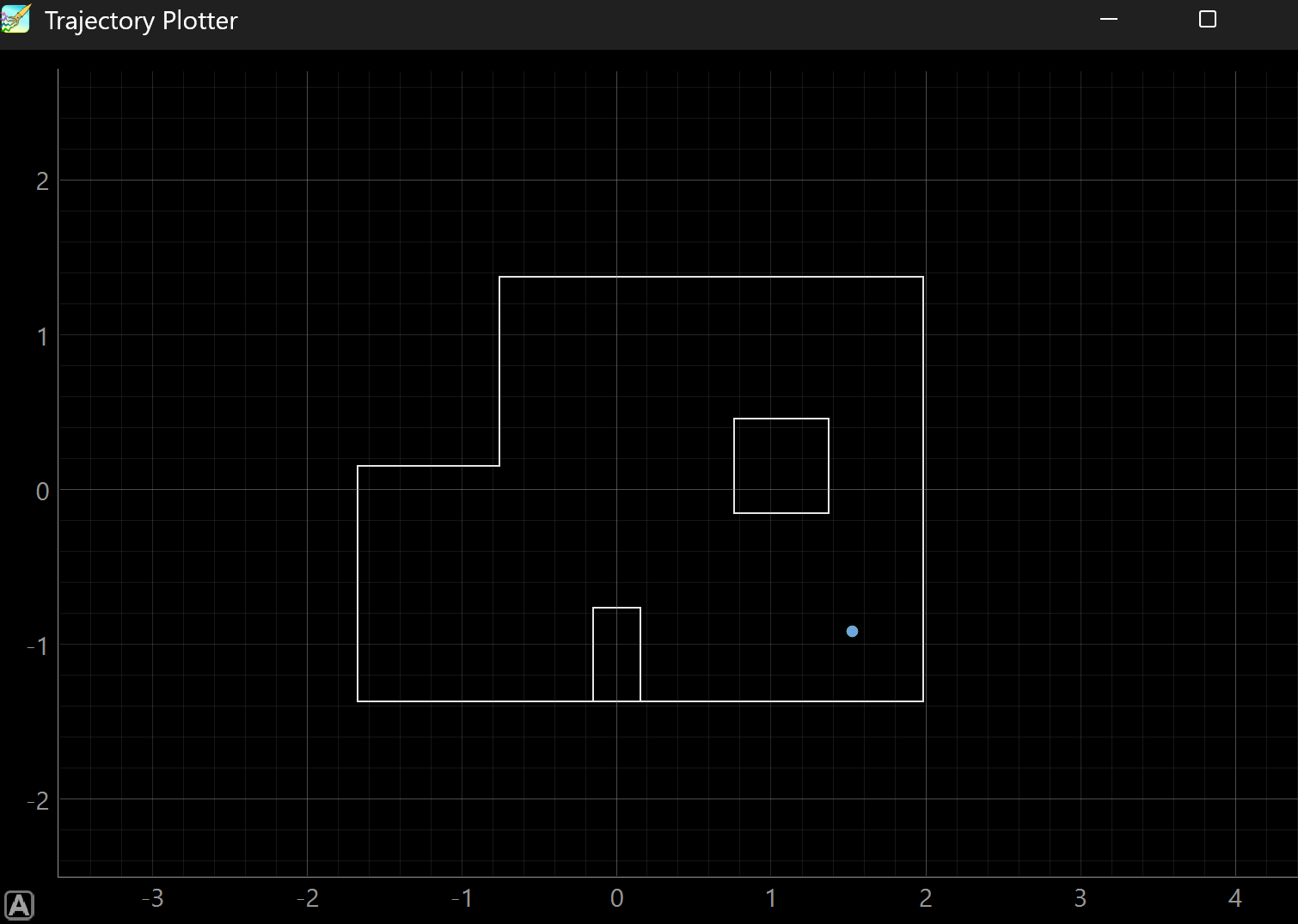
Belief sits exactly on GT in the bottom-right corner. Green dot is hidden under the blue one.

GT (1.524, -0.914), cell (10, 1). Argmax belief on the same cell, perfect localization.

Pose 4: (5 ft, 3 ft, 0°)

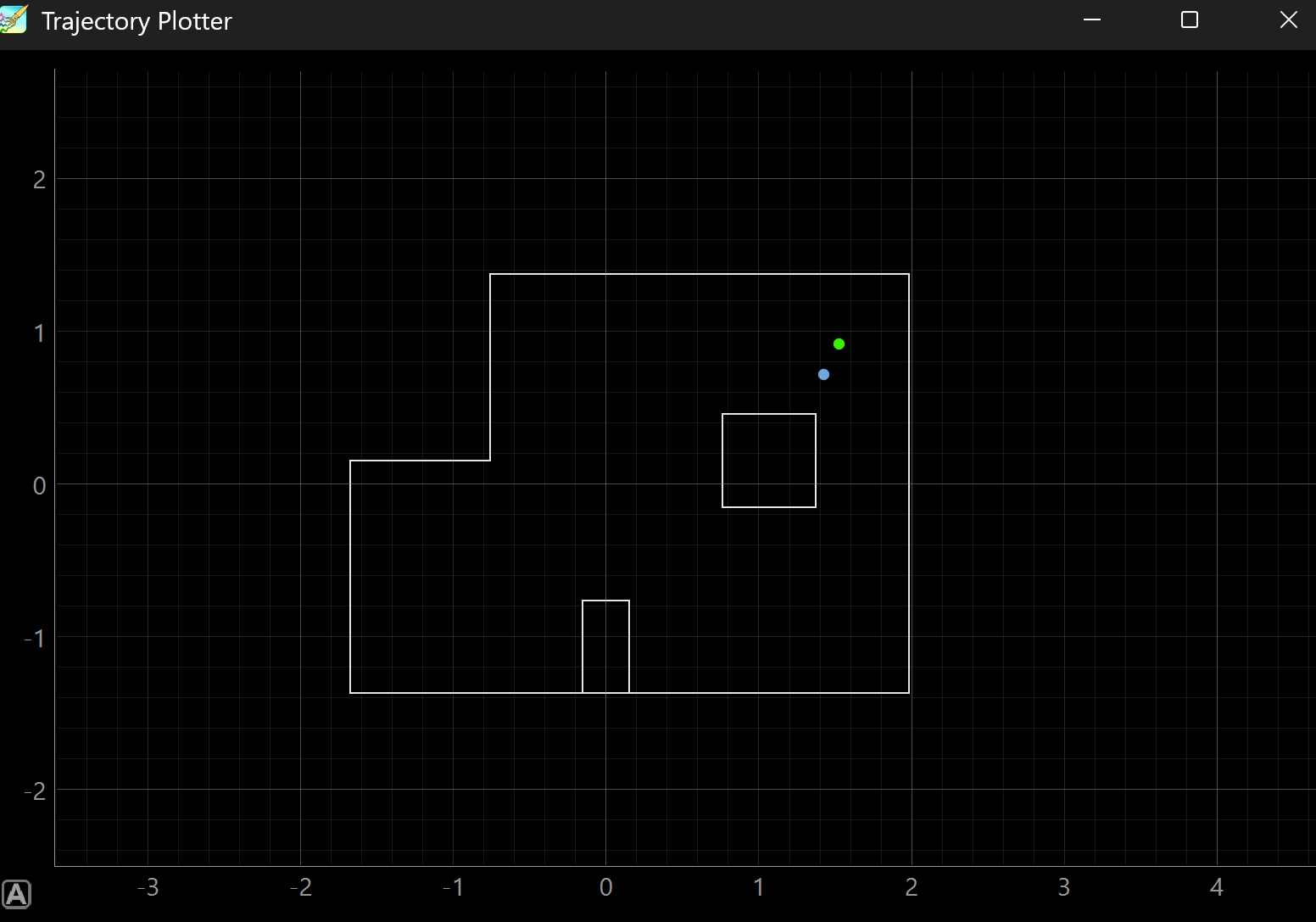
Belief one cell below GT, just above the central box.

GT (1.524, 0.914), cell (10, 7). Belief came back at roughly (1.50, 0.70), close to GT.

Discussion

Two of the four poses (2 and 3) localized exactly on cell, the other two were off by one cell with around 0.2 to 0.36 m error. This roughly matches what Lab 10 produced in simulation, where most steps along the trajectory landed within one cell of GT. The two clean ones were both in distinctive parts of the map. Pose 2 is jammed up in the upper notch with two close walls, pose 3 is wedged into the bottom-right corner with the central box blocking part of the upper view. In both cases the 18 ray fingerprint is sharp enough that no other cell competes.

The two off-by-one poses sat in more open parts of the room. Pose 1 has the long lower wall stretching out to the right along y = -1.37, which is roughly the same distance for several adjacent cells in x, so a small sensor error or a small placement error can slide the argmax one cell over.

The biggest practical lesson was that the two checks before trusting a belief, total yaw delta ≥ 360° and 0 empty bins, are not optional. The pose 3 first-attempt failure had only 2 valid bins and the filter happily produced a probability 1.0 result that was 2 m off GT. The 4 m fallback on empty bins dominates the math very fast.

Skips like the prediction step also feel justified now in a way they didn’t quite in Lab 10. The real odometry from the Artemis with no external position measurement would be guesswork, and the sensor model alone gets to within one cell at three of four poses anyway.